The Next Blockbuster

Objective

There are many aspects to be considered so that a director can make an informed decision regarding the elements — genre, director, star, etc. — of their upcoming film. One aspect they may consider is whether they are motivated by monetary return or artistic value. If they are motivated by monetary return, they may want to identify the genre that has earned the highest gross revenue over the last few decades. On the other hand, if they are motivated by artistic value, they may want to identify the genre that has earned the highest user rating over the last few decades.

Because our stakeholder is Steven Spielberg, I am assuming that he places more value on artistic value as a measure of success. He most likely wants his movie to be remembered as a classic rather than a box office hit. With this assumption and using score — IMDb user rating — I aim to recommend the following to Mr. Spielberg for his upcoming film:

1. The genre
2. A director that has directed films of the determined genre
3. A star that has appeared in films of the determined genre

Data Exploration

Cocktail

Before beginning my exploratory data analysis, I imported the required libraries. Additionally, I set some pandas options, as well as the back end of matplotlib.

# Preparation for pandas and NumPy
import numpy as np
import pandas as pd
from pandas import DataFrame, Series
import matplotlib.pyplot as plt
from matplotlib.pyplot import figure
import seaborn as sns
import plotly.graph_objects as go

# Set some pandas options
pd.set_option('display.notebook_repr_html', False)
pd.set_option('display.max_columns', 30)
pd.set_option('display.max_rows', 30)

# Preparation for matplotlib
%matplotlib inline 

Read in the Data

When trying to read in the CSV file with just pd.read_csv("movies.csv"), the output was a unicode decode error. To resolve the error, I had to manually define the character encoding "ISO-8859-1". Running the following code returns the first five rows, giving us an idea of the data we are working with.

# Read csv file and print first 5 rows
movies = pd.read_csv("movies.csv", encoding = "ISO-8859-1")
movies.head(5)

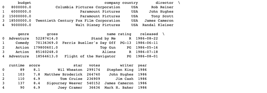movies dataframe

While we can use .head() function to view the first 5 rows, it would be to our best interest to retrieve the full dimensions. Using the DataFrame.shape function, we can see that our data frame is 6,820 by 15. 6,820 observations is more than enough data to conduct our investigation.

# Retrieve the dimensions
print("There are " + str(movies.shape[0]) + " rows and " + str(movies.shape[1]) + " columns in this table.")

Dataframe dimensions

With .dytpes, I can retrieve the data types of all columns. Immediately I learn that most of the columns are of type object, which actually represents strings. This makes sense for columns like company, country, director, etc. I can also see that I am working with a few float and integer data types.

movies.dtypes

Data types

For the purpose of my investigation, I want to view the range of my numerical variables, i.e. columns of type float or integer. I can do so using the .describe() function as follows. Here, we can learn a lot about the data.

movies.describe()

Summary statistics

Data Cleaning

Before moving on, data cleaning is an essential step to any exploratory data analysis. Using the following code retrieves the total number of missing values for each column. From the output, we can see that none of the columns contain any missing values, saving us much of our time and allowing us to continue with our analysis.

movies.iloc[:,:].isnull().sum()

Data cleaning

Subsets of Data

Subset 1: Movies with a Gross in the 75th Percentile

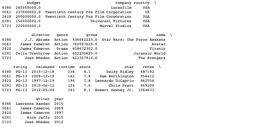
For my first subset, I decided to take the movies with a gross in the 75th percentile, i.e. the gross revenue of these movies are higher than 75% of the movies in this dataframe. Ordering this subset by gross in a descending manner, I can see that although these movies earned a lot in revenue, their scores (although high) do not seem to coincide with their box office success.

This subset may be useful for a producer that has a short term goal of making money fast, but not a producer that has the long term goal of producing films that will be remembered. A director who is motivated by artistic value may want to use score as a measure of success, which I will do in the following subset.

by_gross = movies.loc[movies["gross"] >= 4.006534e+07,:]
by_gross = by_gross.sort_values("gross", ascending=False)
by_gross.head(5)

Subset 1

Subset 2: Movies with a Score in the 75th Percentile

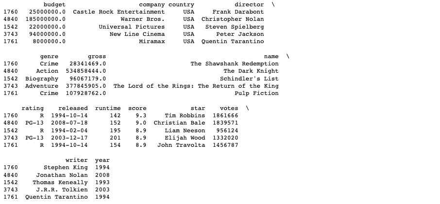
For my second subset, I decided to take the movies with a score in the 75th percentile, i.e. the user ratings of these movies are higher than 75% of the movies in this dataframe. Ordering this subset by score in a descending manner allows producers to view information on the highest rated films.

by_score = movies.loc[(movies["score"] >= 7.1),:]
by_score = by_score.sort_values("score", ascending=False)
by_score.head(5)

Subset 2

Subsetting our data decreased our dimensions from 6,820 by 15 to 1,815 by 15, which is still a good amount of data to draw conclusions from.

by_score.shape

Dataframe dimensions

Subset 3: Genres with a Score in the 75th Percentile

I decided to use by_score to further subset my data so that I could draw specific conclusions. For instance, part of my objective is to recommend the genre for Steven Spielberg’s new movie. To do so, I needed to get a count for each genre that appears in the 75th percentile (based on score). Before I could do that, however, I needed to subset my data into a data frame called by_genres which return the genres with a score in the 75th percentile.

by_genres = by_score[["genre","score"]]
by_genres.head(5)

Subset 3

Subset 4: Directors with a Score in the 75th Percentile

Another aspect of my objective is to recommend a director for Steven Spielberg to work with on his new movie. Again, using by_score, I subsetted the data into a data frame called by_director which returns the director and genre with a score in the 75th percentile.

by_director = by_score[["director","genre","score"]]
by_director.head(10)

Subset 4

Subset 5: Stars with a Score in the 75th Percentile

Additionally, I needed to recommend an actor that will star in Steven Spielberg’s new movie. To do so, using by_score, I subsetted the data into a data frame called by_star which returns the stars with a score in the 75th percentile. I also included the genre of the movie they starred in so that Mr. Spielberg can choose the actor the fits with the recommended genre. It is also worth noting that I only selected stars from the last decade because of their current relevance in Hollywood.

by_star = by_score.loc[by_score["year"] >= 2010,["star","genre","score"]]
by_star.head(10)

Subset 5

Visualization

Pie Chart

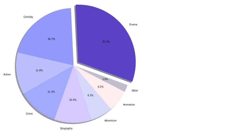
For my first visualization, I wanted to create a pie chart to show the proportion of each genre that is listed in the by_genres subset. Recall that by_genres is a subset of genres that earned a score in the 75th percentile. To do so, I created a dictionary where the first key corresponds to the genre, and the second key correspons to its count.

data = {"Genre":list(by_genres["genre"].value_counts().index),
       "Count":list(by_genres["genre"].value_counts())}

Transforming the dictionary into a dataframe called df, we can see that the 75th percentile is composed of 16 different genres.

df = pd.DataFrame(data)
df

df dataframe

Because I am only interested in genres with a high count, I decided to aggregate the genres with a count below 100 into one row called Other.

total = df[df['Count'] < 100]['Count'].sum()
other = {"Genre":"Other","Count":total}
df = df.append(other, ignore_index=True)

Now when I subset my dataframe with genres that have a count above or equal to total, i.e. the total count of genres with a count below 100, I can see that my dataframe is exactly what I wanted.

df = df.loc[df["Count"]>=total,:]
df

df dataframe

Creating a pie chart from my dataframe df, I can now see the proportion of each genre much more clearly. We can see that Drama movies appear in the 75th percentile the most, followed by Comedy, Action, and so on.

fig = plt.figure(figsize =(10, 10)) 

genres = df["Genre"]
count = df["Count"]
explode = (0.1,) + tuple(np.repeat(0,[len(count)-1]))
colors = ("#5c3ac7","#9495ff","#bbbfff","#a2a7ff","#d6c8ff","#d5d7ff","#ffeeef","#bebfcc")

plt.pie(count, labels=genres, explode=explode, autopct='%1.1f%%', shadow=True, startangle=340, colors=colors)
plt.axis('equal')
plt.show()

Pie chart

Bar Plot

For my second visualization, I wanted to create a bar plot that displays the median score for each genre in the general dataframe movies. To do so, I created another dataframe called grouped_genre that takes the score column and groups it by genre.

grouped_genre = movies['score'].groupby(movies['genre']) 

Using the grouped_genre, I created a dictionary called bar_data where the first key corresponds to the genre and the second key corresponds to the median score. I then use the dictionary to create a dataframe called bar_df that is in ascending order by median score.

bar_data = {"Genre":list(grouped_genre.median().index),
           "Median Score":list(grouped_genre.median())}
bar_df = pd.DataFrame(bar_data)
bar_df = bar_df.sort_values("Median Score", ascending=True)

Creating a bar plot from bar_df, I can see that while Biography films have the highest median score, it is followed by Drama corresponding to what we have seen from the pie chart. Due to the correspondance, Drama seems like the logical genre to choose.

fig = plt.figure(figsize =(18, 10)) 

bar = bar_df.iloc[:,1]
label = list(bar_df["Genre"])

pos = np.arange(len(bar))

plt.barh(pos, bar, align='center', color=['lightgrey','lightgrey','lightgrey','lightgrey','lightgrey','lightgrey',
'lightgrey','lightgrey','lightgrey','lightgrey','lightgrey','lightgrey','lightgrey','lightgrey','lightgrey','crimson',
'lightgrey'])
plt.yticks(pos, label)
plt.xlabel('Median Score')
plt.ylabel('Genre')
plt.title('Median Score by Genre')
plt.show()

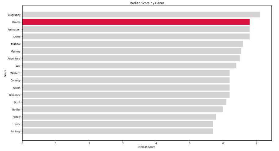Bar chart

Violin Plot

Now that we have chosen the genre, the next step is to choose a director, preferably one who has directed Drama films in the past. To find these potential candidates, I subset my by_director dataframe so that it returns the directors who have directed Drama films that earned a score in the 75th percentile.

drama = by_director[by_director.genre=="Drama"]

Using .values_counts() returns a count for each director. And using .head(5) we can see the 5 directors who have directed the most Drama films that earned a score in the 75th percentile.

drama["director"].value_counts().head(5)

Top Drama Directors

Before I could create my third visualization, I created another dataframe called top_drama that only contains information for the 5 directors listed in the preceding code.

top_drama = drama[(drama.director=="Clint Eastwood")|(drama.director=="Pedro Almodóvar")|
(drama.director=="Ken Loach")|(drama.director=="Richard Linklater")|(drama.director=="Michael Haneke")]

For my third visualization, I created a violin plot that shows the score distribution of the films directed by the top 5 drama directors. Here, we can see that Clint Eastwood has directed movies that have earned the highest scores. He seems like the reasonable candidate to choose.

fig = plt.figure(figsize =(18, 10)) 
vplot = sns.violinplot(x="director", y="score", data=top_drama, palette="Blues", width=1)

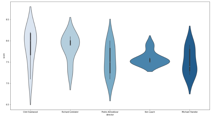Violin Plot

Scatter Plot

The last aspect of my objective is to recommend the leading actor for the film. To do so, I first created a dataframe called actor which is a subset of by_score that consists of star, score, and gross for actors that have appeared in films produced after 2010.

actor = by_score.loc[(by_score["year"] >= 2010) & (by_score["genre"] == "Drama" ),["star","score","gross"]]
actor.head(5)

Actors

For the last visualization, I wanted to create a scatter plot where each point represents the score and gross revenue for each actor. Using the plotly library, I created an interactive scatterplot that enables users to hover over each point and retrieve the name and data values for each star. This plot is particularly useful for directors because they can use both score and gross as criteria in choosing their lead drama actor.

I have a feeling, however, that Steven Spielberg values artistic value over monetary return so he may want an actor that has the highest score regardless of their gross. With this assumption, I’d recommend Mr. Spielberg to consider actor Miles Teller.

plot = go.Figure(data=go.Scatter(x=actor['score'],
                                y=actor['gross'],
                                mode='markers',
                                text=actor['star']))
plot.update_layout(title='Potential Lead Actors for a Drama Movie', xaxis_title="Score", yaxis_title="Gross Revenue")
plot.show()

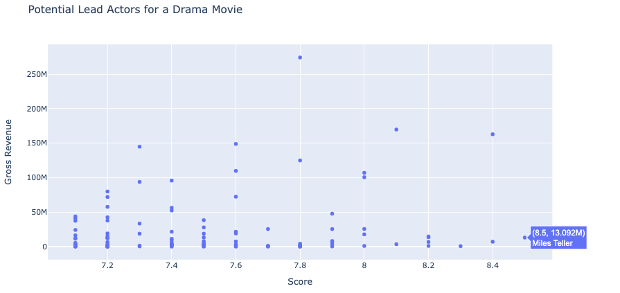Scatter Plot

Summary

In determing the aspects of a new film — genre, director, star, etc. — I had to put my director’s hat on and narrow down the factors a director would consider when making these decisions. The first step would be to identify the source of motivation. Do I have the short term goal of directing a box office hit that earns millions of millions of dollars in gross revenue? Or do I have the long term goal of directing a film that will have the artistry to one day be known as a classic? Steven Spielberg, our stakeholder, has become a household name in Hollywood due to his wide body of work, which includes classics such as E.T. the Extra-Terrestrial, Jaws, and Jurassic Park. With this background, we can assumer that Mr. Spielberg wants his upcoming film to be known as a classic one day.

With this goal, I have decided to use score, the IMDb user rating, to identify the genre, director and star for Mr. Spielberg’s upcoming film. Using score, I created a subset of movies with a score in the 75th percentile called by_score. I chose the 75th percentile as a benchmark because I figured Mr. Spielberg would want his upcoming film to earn a score within the 75th percentile. Using the same benchmark I created a subset called by_genre which returns the genres that lie in the 75th percentile (based on score). Additionally, I created subsets called by_director and by_star which return the directors and stars respectively that lie in the 75th percentile.

Though it is possible for me to determine the genre, director, and star for Mr. Spielberg’s upcoming movie from just the subsets themself, I built several visualizations that would help me make a more informed recommendation. For instance, I built a pie chart visualize the distribution of genres within the 75th percentile. To verify, I also built a bar plot that displays the median score of each genre. Once I selected the genre, I created a violin plot that displays the score distribution of the films directed by the top 5 directors within that genre. Lastly, I created a scatter plot where each point represents the score and gross revenue for each actor. With Mr. Spielberg’s goal, I recommended the actor that earned the highest score regardless of the gross.

Recommendations

When determining the aspects of a new film — genre, director, star, etc. — there are many factors a director must weigh in before making a decision. For instance, they must determine whether they are motivated by monetary return or artistic value. Because our stakeholder is Steven Spielberg, it is safe to assume that he has a long term goal of directing a film that will one day be known as a classic. In this case, it would be to his benefit to identify the genre of the films that received high user ratings.

From our pie chart and bar plot I can conclude that Drama films make up the largest proportion of all genres that lie in the 75th percentile — based on user rating. Using our violin plot, I can also recommend Clint Eastwood as the best option to co-direct since he has produced six drama films with the highest user ratings. Lastly, using our scatter plot, I recommend Mr. Spielberg to consider Miles Teller as his leading actor since the drama film he starred in earned the highest user rating of 8.5.

My official recommendations are as follows,

The source code is available here.