The Direct Line to Reducing Crime

Objective

The objective of this investigation is to identify the cities that exhibit the highest crime and homicide (per capita) growth from 2012 to 2015 within the Western Region of the United States. In doing so, I conducted my research so that it answered the following questions:

Questions of Investigation:

1. What are the top 10 cities with the highest crimes per capita from 2012 and 2015? How do they compare?
2. What are the top 5 cities that exhibited the highest crimes per capita growth?
3. What are the top 5 cities that exhibited the highest homicides per capita growth?

I hope that the executive officers of these cities can use these findings to allocate their resources so they can respond efficiently. Additionally, these findings may help them identify the need for targeted and innovative solutions that would help restore the safety and security of their cities.

Note: The Western Region is composed of the following states: Alaska, Arizona, California, Colorado, Hawaii, Idaho, Montana, Nevada, New Mexico, Oregon, Utah, Washington, Wyoming.

Data Exploration

Cocktail

Before beginning my exploratory data analysis, I imported the required libraries. Additionally, I set some pandas options, as well as the back end of matplotlib.

# Preparation for pandas and NumPy
import numpy as np
import pandas as pd
from pandas import DataFrame, Series
import matplotlib.pyplot as plt
from matplotlib.pyplot import figure

# Set some pandas options
pd.set_option('display.notebook_repr_html', False)
pd.set_option('display.max_columns', 30)
pd.set_option('display.max_rows', 30)

# Preparation for matplotlib
%matplotlib inline 

Read in the Data

The next step to my EDA was to read in the CSV file, using pd.read_csv(), and print the first five rows, using DataFrame.head(n=5). This gives us a glimpse of the dataframe we are working with.

# Read csv file and print first 5 rows
report = pd.read_csv("report.csv")
report.head(5)

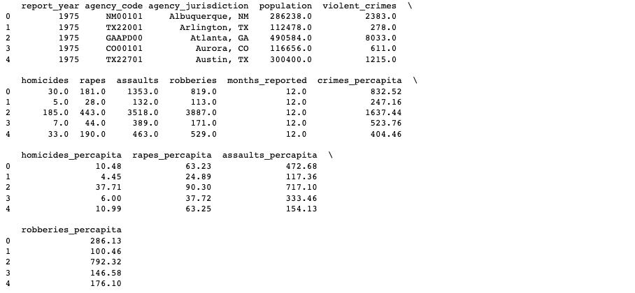report dataframe

While DataFrame.head(n=5) delivers the first 5 rows, I was still interested in the dimensions of the dataframe. To retrieve the dimensions, I utilized the DataFrame.shape method. I now know that I am working with a 2,829 by 15 dataframe.

# Retrieve the dimensions
print("There are " + str(report.shape[0]) + " rows and " + str(report.shape[1]) + " columns in this table.")

Dataframe dimensions

Additionally, I used the DataFrame.columns method to retrieve the column names. Here, I can see all the attributes I am working with. For the purpose of my investigation, I will subset my dataframe, i.e. remove some columns, but I will conduct that in a later step.

# Column names
report.columns

Column names

Because most of my variables are numeric, I was interested in generating a statistical summary of those variables. Using the DataFrame.describe() method, I can see summary statistics of my dataframe. Immediately, I notice that the data collected dates from 1975 to 2015. For the purpose of my investigation, I will subset my data frame with data from my targeted time frame, but I will do so in the following subsection.

report.describe()

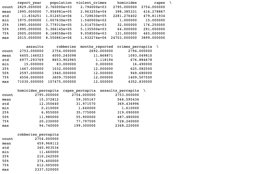Summary statistics

Subset the Data

Because I am only interested in analyzing the crimes and homicides (per capita) of cities within the Western Region from 2012 to 2015, I had to subset the dataframe accordingly. The first line of code subsets the dataframe so that it only contains data for the states that make up the Western Region. The second line of code subsets the dataframe again so that it only contains data pertaining to the crimes and homicides (per capita) committed between 2012 and 2015. The last line of code prints the first 5 lines of our subsetted dataframe, subset.

subset = report[report["agency_jurisdiction"].str.contains("AL|AZ|CA|CO|HI|ID|MT|NV|NM|OR|UT|WA|WY")]
subset = subset.loc[(subset.report_year >= 2012) & (subset.report_year <= 2015),["report_year","agency_jurisdiction", 
        "crimes_percapita", "homicides_percapita"]]
subset.head(5)

Data subset

I decide to look at crimes and homicides (per capita) growth of cities within the Western Region from 2012 to 2015. Using a for loop, I subsetted the crime_report dataframe based on the report_year specified within the loop. The second and third command within the loop adds i, as a string, to the crimes_percapita and homicides_percapita column names to specify the year the data was collected.

The third command within the loop drops the report_year column, as it no longer has much relevance to my investigation. Lastly, the forth command adds the subset to a list called dataframes that will be used to merge all four subsets in the next step.

dataframes = list()

for i in range(2012,2016):
    df = subset.loc[subset.report_year == i,:]
    df.rename(columns={"crimes_percapita":"crimes_percapita" + str(i)}, inplace = True)
    df.rename(columns={"homicides_percapita":"homicides_percapita" + str(i)}, inplace = True)
    df = df.drop("report_year",1)
    
    dataframes.append(df)

I assigned the first subset within dataframes to the variable west_report. Using another for loop, I merged the remaining subsets to the first subset by agency_jurisdiction. This creates a general dataframe that contains the crimes and homicides (per capita) for every Western city between the years 2012 and 2015. Notice that I reset the index to agency_jurisdiction for organizational purposes. Using DataFrame.head(n=5), we can see that west_report is just as we expected.

west_report = dataframes[0]

for i in range(1,(len(dataframes))):
    west_report = pd.merge(west_report, dataframes[i], how = "inner", on = "agency_jurisdiction")
    
west_report = west_report.set_index(['agency_jurisdiction'])
west_report.head(5)

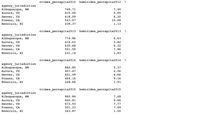Western subset

Just out of curiosity, I wanted to see how much data I was working with now. Following the same steps to retrieve the dimensions, I can now see that I am looking at the crimes (per capita) records of 20 cities.

# Retrieve the dimensions
print("There are " + str(west_report.shape[0]) + " rows and " + str(west_report.shape[1]) + " columns in this table.")

Dataframe dimensions

Data Cleaning

Before moving on to conduct further analysis, it is essential that I check my west_report dataframe for any missing or null values. The following code retrieves the sum of missing values for each column. Here I can see that crimes_percapita2015 and homicides_percapita2015 contains one missing value.

west_report.iloc[:,:].isnull().sum()

Missing values

Using the DataFrame.dropna() method, I removed the one row containing missing values. Following the same code as above, I can verify that west_report no longer contains any missing values.

west_report = west_report.dropna()
west_report.iloc[:,:].isnull().sum()

Clean dataset

Additionally, we can check the dimensions to verify that the one row containing missing values was removed. Indeed, I can see that I am now working with data for 19 cities.

# Retrieve the dimensions
print("There are " + str(west_report.shape[0]) + " rows and " + str(west_report.shape[1]) + " columns in this table.")

Dataframe dimensions

One Column Selection

I am interested in finding the top 10 cities with the highest crimes per capita from 2012. To do so, I sorted the west_report dataframe where the rows are in descending order based on the crimes_percapita2012 column.

Printing the first 10 rows delivers the cities with the highest crimes per capita from 2012.

west_report.sort_values("crimes_percapita2012", ascending=False).iloc[0:10,0]

Top 10 crime-ridden cities (2012)

Since my investigation is focused on analyzing the growth in crimes (per capita), I am interested in whether the 10 cities found above maintained these spots in 2015 as well. Following the same steps above but using the crimes_percapita2015 column, we can see that while there is a little shuffling, the same cities are indeed listed.

west_report.sort_values("crimes_percapita2015", ascending=False).iloc[0:10,6]

Top 10 crime-ridden cities (2015)

Sort

Currently, the west_report dataframe consists of eight columns that document the crimes and homicides (per capita) that occured in Western cities for each year between 2012 and 2015. Part of my objective is to analyze the crime and homicide (per capita) growth between 2012 and 2015. To capture the growth, I created two more columns called Crime_Percent_Change and Homicide_Percent_Change.

west_report["Crime_Percent_Change"] = ((west_report["crimes_percapita2015"] - west_report["crimes_percapita2012"]) / 
west_report["crimes_percapita2012"])*100

west_report["Homicide_Percent_Change"] = ((west_report["homicides_percapita2015"] - 
west_report["homicides_percapita2012"]) / west_report["homicides_percapita2012"])*100

Additionally, I created another subset called sort_by_crime that contains data pertaining to the crime per capita where the rows are in descending order based the Crime_Percent_Change column.

sort_by_crime = west_report.iloc[:, [0,2,4,6,8]]
sort_by_crime = sort_by_crime.sort_values("Crime_Percent_Change", ascending = False)

Printing the first five rows delivers the cities with the highest crime per capita growth from 2012 to 2015.

sort_by_crime.head(5)

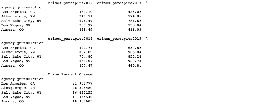Top 5 cities with the highest crime growth

Series

Lets take a look at what the west_report data frame looks like now.

west_report.head(3)

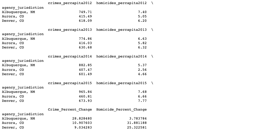west_report dataframe

Since I have already captured the crime per capita growth, I now want to capture the homicide per capita growth. To do so, I subsetted the west_report dataframe into another dataframe called homicide_report that contains data pertaining to the homicides per capita.

homicides_report = west_report.iloc[:, [1,3,5,7,9]]

Lets print the first 5 rows to verify.

homicides_report.head(5)

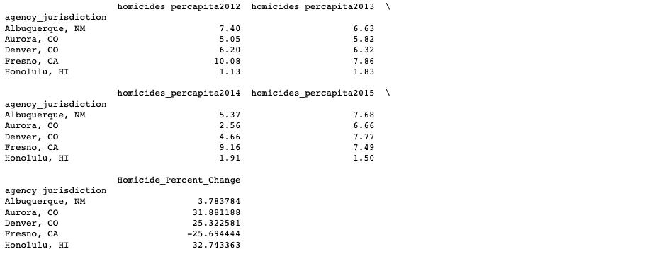homicides_report dataframe

Using the DataFrame.describe() method, I retrieved a statistical summary of each of the 5 columns. From here, I can see that the average homicides per capita portrayed a steady decrease from 2012 to 2014 but exhibited a sudden jump from 2014 to 2015. Additionally, the median of Homicide_Percent_Change is near 0, indicating that half of the cities saw a decrease in homicides from 2012 to 2015 while the other half saw an increase from 2012 to 2015.

homicides_report.describe()

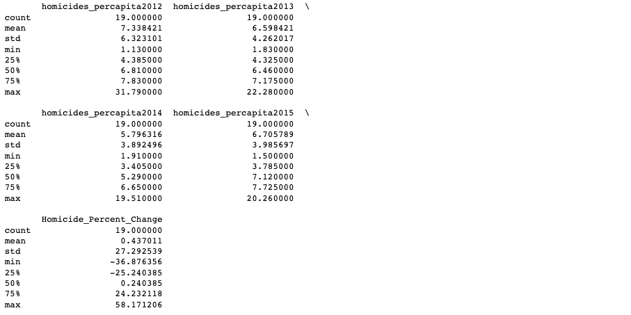Summary statistics

Similar to crimes per capita, I am interested in the cities with the highest homicides per capita growth from 2012 to 2015. To find these, I created another subset called sort_by_homicide where the rows are in descending order based the Homicide_Percent_Change column.

sort_by_homicide = homicides_report.sort_values("Homicide_Percent_Change", ascending = False)

Printing the first five rows delivers the cities with the highest homicide per capita growth from 2012 to 2015.

sort_by_homicide.head(5)

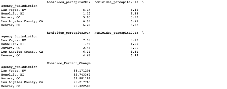sort_by_homicide dataframe

Plot

Though I can observe the crime and homicide (per capita) growth from their corresponding columns, a grouped bar plot can deliver a better visualization. To plot the data, I created a function called bar_plot() that takes in two arguments — the first being a specified dataframe and the second being a specified attribute. Running the function will plot the 2012 and 2015 records for the first five cities listed in the dataframe.

def bar_plot(df, attribute):
    x = df.head(5)
    
    figure(num=None, figsize=(16, 7))
    
    bar1 = x.iloc[:,0]
    bar2 = x.iloc[:,3]
    
    label = [x.index[0], x.index[1], x.index[2], x.index[3], x.index[4]]
    
    pos1 = np.arange(len(bar1))
    pos2 = pos1 + 0.2
    
    plt.bar(pos1, bar1, width = 0.25, color = "skyblue", label = "2012")
    plt.bar(pos2, bar2, width = 0.25, color = "navy", label = "2015")
    
    plt.xticks(pos1, label)
    plt.xlabel("County")
    plt.ylabel(str(attribute) + " per Capita")
    plt.title("Top " + str(attribute) + " Jumps in Western Region" )
    plt.legend()
    plt.show()

The code below runs the bar_plot() function using the sort_by_crime dataframe and the crimes (per capita) attribute. Now we can visually see tthe cities that had the highest crime (per capita) growth from 2012 to 2015.

bar_plot(sort_by_crime, "Crime")

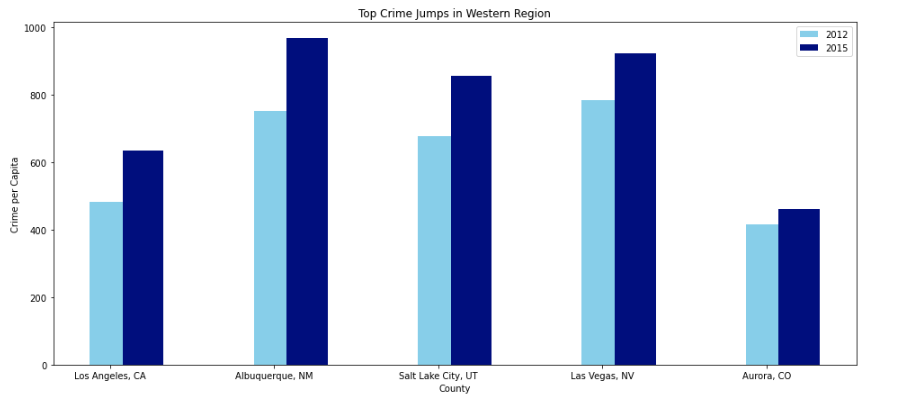sort_by_crime bar plot

The code below runs the bar_plot() function using the sort_by_homicide dataframe and the homicides (per capita) attribute. Now we can visually see the the cities that had the highest homicide (per capita) growth from 2012 to 2015.

bar_plot(sort_by_homicide, "Homicide")

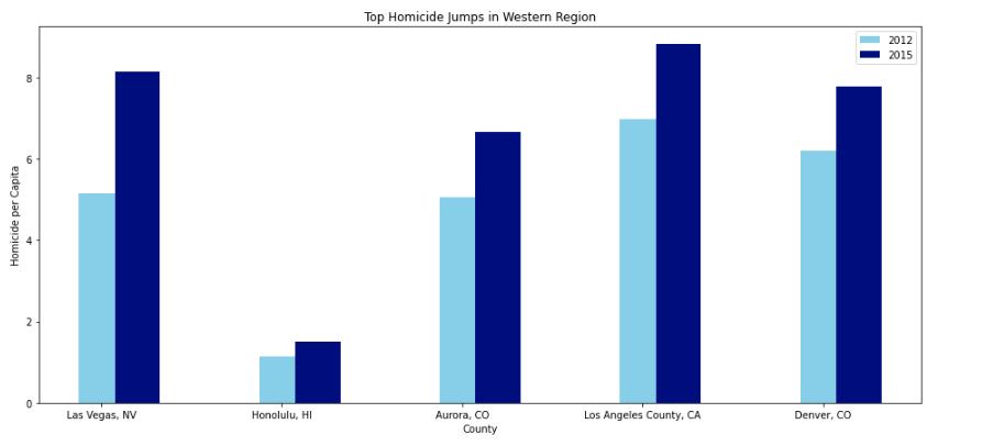sort_by_homicide bar plot

Summary

In observing the growth in crime across different locations and times, I had to aggregate my data in such a manner that would allow me to do so. I decided to narrow my study so that I could identify the cities within the Western Region of the United States that exhibited the highest growth in crimes and homicides per capita from 2012 to 2015. In doing so I created a subsetted dataframe, west_report, that contains the yearly crime and homicide (per capita) report for every Western city between the years 2012 and 2015. Additionally, I created two more columns called that indicate the crime and homicide (per capita) growth between 2012 and 2015. Now, with this subset, I was able to answer all of my questions of investigation.

What are the top 10 cities with the highest crimes per capita from 2012 and 2015? How do they compare?
To find the top 10 cities with the highest crimes per capita from 2012, I sorted the west_report dataframe where the rows are in descending order based on the crimes_percapita2012 column. To find the top 10 cities with the highest crimes per capita from 2015, I followed the same steps but with the crimes_percapita2015 column. Printing the first 10 rows of each, I learned while there is a little shuffling, the same 10 cities were found in both listings.

What are the top 5 cities that exhibited the highest crimes per capita growth?
To capture the crime per capita growth, I created another subset from west_report called sort_by_crime that contains data pertaining to the crime per capita where the rows are in descending order based on crime per capita growth. Printing the first five rows, I can see that the top five cities that exhibited the highest crime per capita growth are Los Angeles, CA, Alburqueque, NM, Salt Lake City, UT, Las Vegas, NV, and Aurora, CO,

What are the top 5 cities that exhibited the highest homicides per capita growth?
To capture the homcide per capita growth, I followed a similar procedure as above. I created another subset from west_report called sort_by_homicide that contains data pertaining to the crime per capita where the rows are in descending order based on homicide per capita growth. Printing the first five rows, I can see that the top five cities that exhibited the highest homicide per capita growth are Las Vegas, NV, Honolulu, HI, Aurora, CO, Los Angeles County, CA, and Denver CO.

Recommendations

When deploying police enforcement, there are many factors law enforcement agencies must consider so that they can optimize the allocation of the available resources. For instance, it would be to the benefit of executive officers to know which cities exhibited the highest growth in crime between a specified period. Knowing this information allows officers to respond efficiently by identifying targeted and innovative solutions.

Based on my findings, I recommend that the executive officers of the cities that exhibited the highest crime growth (per capita) from 2012 to 2015 to take a second look at their resource budget and determine whether they can allocate more funding to targeted services that could reduce the number of crimes committed in their city. Additionally, they may want to focus on the conditions that drive people into criminal and unlawful behavior. This may require an examination of the systemic and societal conditions within these cities.

While the recommendations from above can be applied to any type of crime, reducing a specific type of crime may require a more targeted solution. Take the cities that exhibited the highest homicide growth (per capita) from 2012 to 2015 for instance. If the executive officers of these cities are looking to reduce homicides, they may want to explore the idea of programmes that target the population group that is most likely to commit this type of crime. Additionally, they may want to identify and diagnose the risk factors that drive this population into criminal activity. A treatment plan, complemented with the support of the family and community, could deliver significant results.

The source code is available here.